- Vinay Anant
- Dec 7, 2021
- 3 min read
Fake news is information that is not true, i.e., it is inaccurate information that can be used to spread misleading information, perhaps leading to unforeseeable outcomes.
Here we are building a classifier that can determine whether news is real or fake.
The dataset that has been used for this classifier is available here.
Import libraries
First we are importing necessary libraries which includes numpy pandas, matplotlib, scikit learn and many more.
Import dataset
Here we are importing the dataset which can be imported using pandas. Also drop any na values from the dataset to make it cleaner.

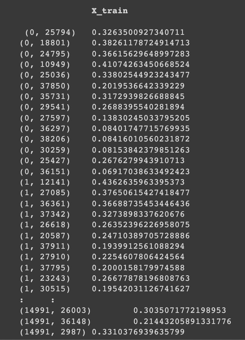
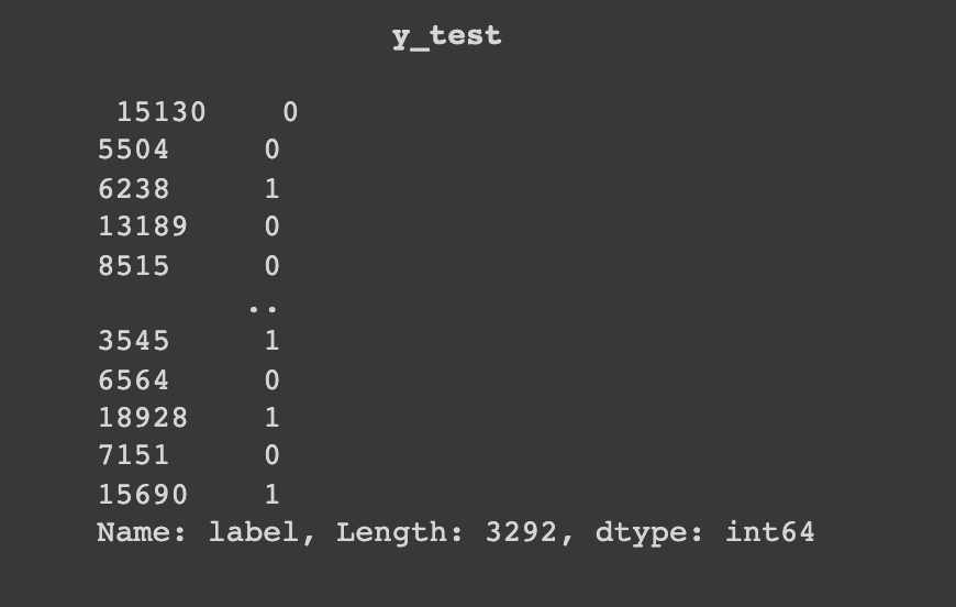
Splitting the dataset
Now we are splitting the dataset into training and test. Here it can be any value which gives us an accurate result i.e. 80:20 split i.e. 80 for training and 20 for testing.


Train and test using various models
Let's make a function that consists of training the model so that it can offer us with the necessary accuracy on the test set.
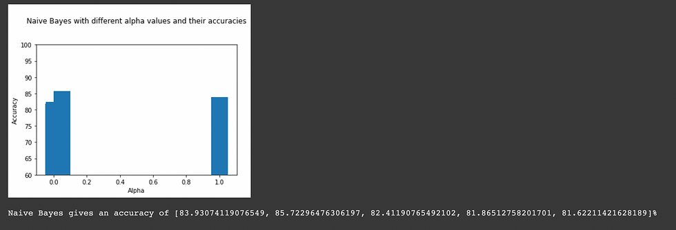
Naive Bayes Classifier
MultinomialNB implements the naive Bayes algorithm for multinomially distributed data, and is one of the two classic naive Bayes variants used in text classification (where the data are typically represented as word vector counts, although tf-idf vectors are also known to work well in practice). The distribution is parametrized by vectors θy=(θy1,…,θyn) for each class y, where n is the number of features (in text classification, the size of the vocabulary) and θyi is the probability P(xi∣y) of feature appearing in a sample belonging to class y.
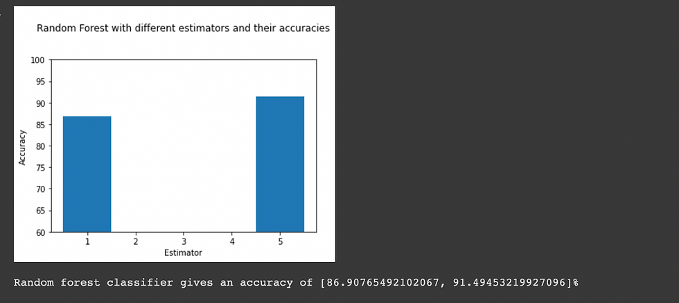
Random Forest Classifier
Random forest is a meta estimator that fits a number of decision tree classifiers on various sub-samples of the dataset and uses averaging to improve the predictive accuracy and control over-fitting. The sub-sample size is controlled with the max_samples parameter if bootstrap=True (default), otherwise the whole dataset is used to build each tree.
Logistic Regression
Logistic Regression implements regularized logistic regression using the ‘liblinear’ library, ‘newton-cg’, ‘sag’, ‘saga’ and ‘lbfgs’ solvers. Note that regularization is applied by default. It can handle both dense and sparse input. Use C-ordered arrays or CSR matrices containing 64-bit floats for optimal performance; any other input format will be converted.

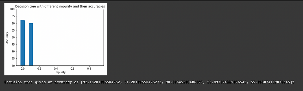
Decision Tree
Decision Trees are a non-parametric supervised learning method used for classification and regression. The goal is to create a model that predicts the value of a target variable by learning simple decision rules inferred from the data features. A tree can be seen as a piecewise constant approximation.
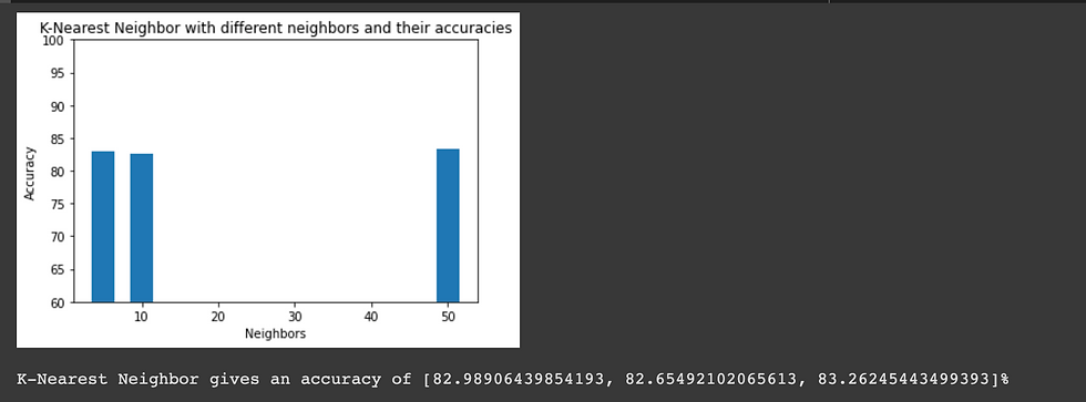
K-Nearest Neighbor
Neighbors-based classification is a type of instance-based learning or non-generalizing learning: it does not attempt to construct a general internal model, but simply stores instances of the training data. Classification is computed from a simple majority vote of the nearest neighbors of each point: a query point is assigned the data class which has the most representatives within the nearest neighbors of the point.
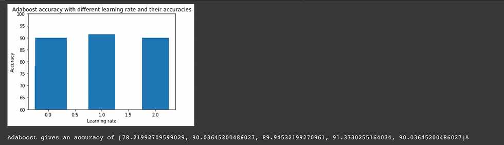
AdaBoostClassifier
AdaBoost classifier is a meta-estimator that begins by fitting a classifier on the original dataset and then fits additional copies of the classifier on the same dataset but where the weights of incorrectly classified instances are adjusted such that subsequent classifiers focus more on difficult cases.
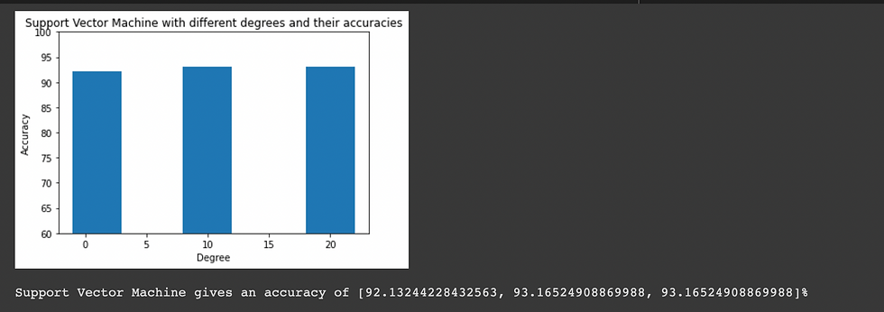
Support Vector Machine
Support Vector Machine finds a hyperplane in an N-dimensional space(N — the number of features) that distinctly classifies the data points.
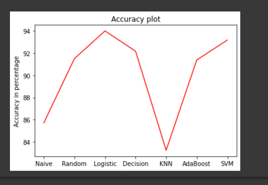
Comparison and visualization of different models accuracies

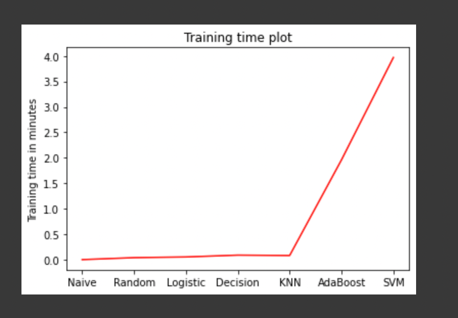
Training time comparison and visualization of different models

Conclusion
As we can see that the maximum accuracy has been achieved by logistic regression which is 93.9854191980559%.
Experiments and findings
Experimented with over 6 different models, including naive bayes, random forest, logistic regression, decision tree, KNN, adaboost and SVM, as well as hyper parameter tuning. The discovery is that utilizing logistic regression with less training time, the best accuracy above 93 percent has been achieved.
Overfitting has not been observed in the above models as we have supplied an ample amount of data.
Challenges
The challenge was to enhance accuracy, which was accomplished by conducting numerous tests in test-train split, implementing multiple models, and experimenting with their various hyperparameters.
Contribution
Understood the code from this link and extended it for 7 different models including naive bayes, random forest, logistic regression, decision tree, KNN, adaboost , SVM and performed various hyperparameter tuning, yielding an accuracy of more than 93 percent with logistic regression
Visualization and comparison of accuracy and training time for above models using various types of plots
This notebook can be found here
The demo of this project can be found here
Please note that the algorithm explanation has been referred from the links which is embedded on the first word of every explanation.
References:


